When you are looking for more than one of a single entry in Google Sheets, just the thought screams “time-consuming” in your head. If, for example, you are trying to find out how many times the word “Brown” appeared on your spreadsheet, you could spend half the day looking at a large spreadsheet with thousands of entries trying to sort that data. Or, you could use conditional formatting to highlight duplicates in Google Sheets and get the answer in just a few seconds.
If you’ve never used conditional formatting before, you don’t know what time-saving lessons you are missing for Google Sheets. Learn more about conditional formatting in Google Sheets and how it can speed your workflow up permanently.
Learn About Conditional Formatting
Conditional formatting is a feature of Google Sheets that allows you to highlight duplicates in a spreadsheet to organize your work faster and more efficiently. You will save time using conditional formatting, and you will have better answers from your work when you use it, because you will be less likely to make human errors when calculating duplicates.
Conditional formatting allows you to apply highlighted colors to specific cells in your Google Sheets so that you can see answers instantly, without having to hunt for them. You decide the rules and how that sounds, and it is all based on if/then formatting formulas. For example, you tell Google Sheets, “if G18 is Brown then make that cell a green color”.
You can apply that to an entire range of cells, an entire spreadsheet, and decide why a cell looks the way that it does. For conditional formatting rules, you need the range of cells, the value you want to highlight, and the style you want to highlight, and that’s it.
Let’s try an example.
One Column: Highlight Duplicates in Google Sheets
If you can handle highlighting duplicates in Google Sheets in a single column, it won’t take you long to do longer and more complicated ranges. The goal here is to save time. You are also looking for duplicates, so you are looking for “more than 1” of something.
Use one of your Google Sheets as practice, where you have the same value entered a few times. Select the range of one column with your cursor, the same way you would sum that column. Let’s say, for example, you are looking for duplicates of the word “Brown” in column E, with the first instance appearing in E1, but you want to use your own value here.
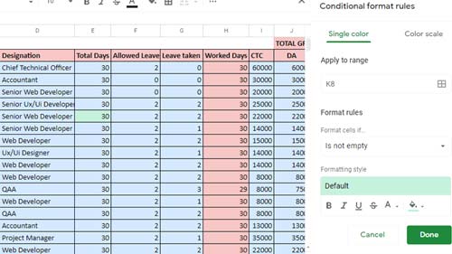
With the column selected, click on Format, and then Conditional formatting. This brings you to a drop-down menu. Here you can create a custom formula so that you know your formatting will be specified to your rules. Click on the drop-down menu for “Format cells if” and at the bottom of the drop-down menu is an option “Custom formula is” and a space to enter a value. Enter: =countif(E1:E, E1)>1. Now, click on Formatting style and decide what color you want those cells to be.
Here you are asking Google Sheets to highlight Brown when there is more than one of them on the sheet. Click Done and your duplicates should be highlighted.
Let’s do this in multiple columns now.
Multiple Columns: Highlight Duplicates in Google Sheets
Now you are going to do the exact same thing, but you are going to have a few different formulas here. So let’s say you are still looking for Brown, but it might be in another column as well.
Click on Format, and then Conditional formatting again. Click on Format rules, select Custom formula is from the bottom of the dropdown menu. Start with the same formula, but specify the range of columns (from columns E to G, for example) you are searching in: =countif(E1:G,E1)>1. You will then select your highlighting formatting and click done.
In this example, E1 is the first instance of the word Brown, and using E1 twice in this formula is an easy way of telling Google Sheets you are looking for more than one instance of the word Brown in this many columns, and you want them highlighted this color.
You can highlight duplicates in multiple columns for the whole spreadsheet the same way. Let’s say Brown appears in B1, but could appear in Z 222, the last used cell on the spreadsheet. Your custom formula here then would be =countif(B1:Z,B1)>1. In Formatting style, select the color that you want for that, click Done, and you’ve just highlighted duplicates in multiple columns.
Learn to Highlight Duplicates in Google Sheets
When you are looking for the same thing over and over in Google Sheets, use conditional formatting. It is so much faster to highlight duplicates in Google Sheets than it is to spend the day highlighting every entry of the word “Brown” manually. Conditional formatting saves time and will make your workday go faster.